RNA-Seq Analysis Pipeline: From Raw Data to Functional Enrichment
This guide outlines a standardized, reproducible pipeline for RNA-seq data analysis. It is divided into two main sections:
- Upstream Analysis: Processing raw sequencing data in a Linux environment.
- Downstream Analysis: Statistical modeling and visualization using R.
Table of Contents
Part 1: Upstream Analysis (Linux Environment) 🐧
1. Environment & Directory Structure
Software Prerequisites: To ensure reproducibility and avoid dependency conflicts, it is highly recommended to use Conda (or the faster Mamba) for environment management.
- fastp: An ultra-fast all-in-one FASTQ preprocessor (QC + Trimming).
- STAR: Spliced Transcripts Alignment to a Reference (Industry standard aligner).
- subread: A package containing
featureCountsfor efficient quantification. - samtools: The swiss-army knife for BAM/SAM file manipulation.
Step 1: Setup Conda Environment:
Run the following commands to create a dedicated environment and install all necessary tools from the bioconda channel.
# 1. Create a new environment named 'rnaseq'
conda create -n rnaseq

# 2. Activate the environment
conda activate rnaseq

# 3. Install software (Using mamba is recommended for speed, but conda works too)
# We explicitly specify channels to ensure correct versions
conda install -c bioconda -c conda-forge fastp star subread samtools

# 4. Verify installation
fastp --version
STAR --version
featureCounts -v
samtools --version
Step 2: Directory Initialization: A clean folder structure is the foundation of reproducible research. Run the following commands in your project root to initialize the workspace:
# Create standard directory structure
mkdir -p 00.RawData    # Store raw FASTQ files here
mkdir -p 01.CleanData  # Store filtered/trimmed FASTQ files
mkdir -p 02.Genome     # Store reference genome (FASTA) and annotation (GTF)
mkdir -p 03.Align      # Store alignment results (BAM files)
mkdir -p 04.Counts     # Store final expression matrix
2. Reference Preparation
You need to download the reference genome (FASTA) and the gene annotation file (GTF). Common sources include Ensembl, GENCODE, or UCSC.
- FASTA (.fa): The actual DNA sequence of the genome.
- GTF (.gtf): The map telling software where genes, exons, and transcripts are located.
cd 02.Genome

# Download hg38 (GRCh38) genome sequence
wget https://ftp.ebi.ac.uk/pub/databases/gencode/Gencode_human/release_49/GRCh38.primary_assembly.genome.fa.gz

# Download corresponding annotation
wget https://ftp.ebi.ac.uk/pub/databases/gencode/Gencode_human/release_49/gencode.v49.annotation.gtf.gz

# Decompress files (STAR requires uncompressed FASTA usually)
gunzip *.gz
3. Build Index
Before alignment, STAR must generate a genome index. This step is computationally intensive but only needs to be performed once per genome version.
# Ensure you are in the 02.Genome directory
STAR --runMode genomeGenerate \
     --runThreadN 16 \
     --genomeDir ./star_index \
     --genomeFastaFiles GRCh38.primary_assembly.genome.fa \
     --sjdbGTFfile gencode.v49.annotation.gtf \
     --sjdbOverhang 149
📝 Parameter Explanation:
--runMode genomeGenerate: Switches STAR to index-building mode (default is alignment mode).--runThreadN 16: Uses 16 CPU threads. Adjust this based on your server’s capacity to speed up the process.--genomeDir ./star_index: Specifies the output directory for the index files.--sjdbGTFfile: Providing the GTF file here improves alignment accuracy specifically across splice junctions.--sjdbOverhang 149: Critical Parameter. Ideally set toReadLength - 1. For standard Illumina PE150 (150bp) sequencing, use 149. If you have PE100 data, set this to 99.
❓ How to determine the correct
sjdbOverhang?The general formula is:
Read Length - 1.If you are unsure about your sequencing read length (e.g., PE150 vs PE100), use one of the following methods:
- Method A (Check Report): Open the
fastp.htmlreport generated in Step 4 (run fastp first if needed). Look at the “Summary” table -> “Read1 before filtering” -> “mean length”.- Method B (Command Line): Run this command to directly count the length of the first read in your raw data:
# Print the length of the first sequence line zcat ../00.RawData/Sample1_1.fq.gz | head -n 2 | tail -n 1 | awk '{print length}'- Common Values:
- If output is 150 (Standard Illumina PE150) $\rightarrow$ set overhang to 149.
- If output is 100 (Illumina PE100) $\rightarrow$ set overhang to 99.
4. QC & Trimming
We use fastp because it performs quality control and adapter trimming in a single pass, making it significantly faster than combining FastQC and Trimmomatic.
Assuming Paired-End (PE) data named Sample1_1.fq.gz and Sample1_2.fq.gz:
cd ../01.CleanData

fastp -i ../00.RawData/Sample1_1.fq.gz \
      -I ../00.RawData/Sample1_2.fq.gz \
      -o Sample1_1.clean.fq.gz \
      -O Sample1_2.clean.fq.gz \
      -h Sample1.fastp.html \
      -j Sample1.fastp.json \
      --detect_adapter_for_pe \
      -w 8
📝 Parameter Explanation:
-i / -I: Input files (Read 1 and Read 2).-o / -O: Output cleaned files.-h: Generates a visual HTML report. Always download and open this file to check sequencing quality, duplication rates, and adapter content.--detect_adapter_for_pe: Automatically detects and trims adapter sequences without needing manual input.-w 8: Uses 8 threads for parallel processing.
5. Alignment
This is the core step where cleaned reads are mapped to the genome index.
cd ../03.Align

STAR --runThreadN 16 \
     --genomeDir ../02.Genome/star_index \
     --readFilesIn ../01.CleanData/Sample1_1.clean.fq.gz ../01.CleanData/Sample1_2.clean.fq.gz \
     --readFilesCommand zcat \
     --outFileNamePrefix Sample1_ \
     --outSAMtype BAM SortedByCoordinate \
     --outBAMsortingThreadN 8 \
     --quantMode GeneCounts
📝 Parameter Explanation:
--readFilesCommand zcat: Tells STAR that input files are gzipped (.gz), so it useszcatto read them on the fly.--outSAMtype BAM SortedByCoordinate: Highly Recommended. Directly outputs a binary BAM file sorted by genomic coordinates. This saves disk space (vs SAM) and saves time (skips manual sorting withsamtools sort).--quantMode GeneCounts: Outputs a basicReadsPerGene.out.tabcount file. While we will use featureCounts later, this provides a quick “sanity check” to ensure mapping worked.
6. Quantification
Finally, we count how many reads map to each gene using featureCounts from the Subread package.
cd ../04.Counts

# Quantify all BAM files in the Align directory at once
featureCounts -T 16 \
              -p \
              -t exon \
              -g gene_id \
              -a ../02.Genome/gencode.v49.annotation.gtf \
              -o all_counts.txt \
              ../03.Align/*.bam
📝 Parameter Explanation:
-T 16: Usage of 16 threads.-p: Crucial for PE data. Specifies that the input is Paired-End. Do not use this for Single-End data.-t exon: Specifies the feature type to count. We count reads aligning toexonregions.-g gene_id: Specifies the attribute type to summarize by. We want counts pergene_id(meta-feature), grouping all exons belonging to one gene.../03.Align/*.bam: The wildcard*allows processing all samples simultaneously, creating a single merged expression matrix.
Part 2: Downstream Analysis (R Environment) 📊
Once you have generated all_counts.txt and prepared your metadata.txt (sample grouping info), switch to RStudio.
1. Setup & Data Import
# Install packages if missing
# BiocManager::install(c("DESeq2", "tidyverse", "pheatmap", "clusterProfiler", "org.Hs.eg.db"))

library(DESeq2)
library(tidyverse)

# 1. Load Data
counts_data <- read.table("counts.txt", header=TRUE, row.names=1, sep="\t")
colnames(counts_data) <- gsub("\\.\\.\\.03\\.Align\\.|_Aligned\\.sortedByCoord\\.out\\.bam", "", colnames(counts_data))
counts_data <- counts_data[,6:ncol(counts_data)]

col_data <- read.table("metadata.txt", header=TRUE, row.names=1, sep="\t")

# Sanity Check: Verify consistency between data and metadata
# The rows of metadata MUST match the columns of count data exactly
if(!all(rownames(col_data) == colnames(counts_data))) {
  stop("Error: Sample names in col_data and counts_data do not match!")
}

# 2. Set Factors
# Define the reference level for comparison (e.g., Control/Mock)
col_data$Condition <- factor(col_data$Condition, levels = c("Mock", "Infected"))
2. DESeq2 Workflow
We use DESeq2 for differential expression analysis as it robustly handles biological variability and low-count genes.
# Construct DESeqDataSet Object
dds <- DESeqDataSetFromMatrix(countData = counts_data,
                              colData = col_data,
                              design = ~ Condition)

# Pre-filtering: Remove rows with very low counts
# This reduces the size of the object and increases calculation speed
keep <- rowSums(counts(dds)) >= 10
dds <- dds[keep, ]

# Run the full differential expression pipeline
dds <- DESeq(dds)
3. QC: Principal Component Analysis (PCA)
PCA projects high-dimensional data into 2D space. It is the best tool to visualize sample clustering and detect potential outliers or batch effects.
# Variance Stabilizing Transformation (VST)
# VST normalizes data so that variance is not dependent on the mean
vsd <- vst(dds, blind=FALSE)

# Plot PCA
plotPCA(vsd, intgroup="Condition")
4. Extract Differentially Expressed Genes (DEGs)
# Extract results: Infected vs Mock
res <- results(dds, contrast=c("Condition", "Infected", "Mock"))

# LFC Shrinkage
# Shrinks log2 fold changes for genes with low expression or high dispersion
# This provides more accurate rankings for visualization
resLFC <- lfcShrink(dds, contrast=c("Condition", "Infected", "Mock"), type="normal")

# Convert to Dataframe for filtering
res_df <- as.data.frame(resLFC)

# Filter Significant Genes
# Common threshold: Adjusted P-value < 0.05 and Fold Change > 2 (|log2FC| > 1)
sig_genes <- res_df %>%
  filter(padj < 0.05 & abs(log2FoldChange) > 1)

# Save results
write.csv(sig_genes, "Diff_Genes_Infected_vs_Mock.csv")
5. Visualization
A. Volcano Plot 🌋
Visualizes the relationship between statistical significance (padj) and magnitude of change (log2FoldChange).
library(ggplot2)

# Annotate Up/Down regulation for coloring
res_df$diff <- "NO"
res_df$diff[res_df$log2FoldChange > 1 & res_df$padj < 0.05] <- "UP"
res_df$diff[res_df$log2FoldChange < -1 & res_df$padj < 0.05] <- "DOWN"

# Plot
ggplot(res_df, aes(x=log2FoldChange, y=-log10(padj), color=diff)) +
  geom_point(alpha=0.5) +
  theme_minimal() +
  scale_color_manual(values=c("blue", "grey", "red")) +
  geom_vline(xintercept=c(-1, 1), lty=2, color="black") +
  geom_hline(yintercept=-log10(0.05), lty=2, color="black") +
  labs(title = "Volcano Plot", x = "log2 Fold Change", y = "-log10(Adjusted P-value)")
B. Heatmap 🔥
Visualizes the expression patterns of significant genes across all samples.
library(pheatmap)

# Extract expression matrix for only the significant genes
sig_gene_names <- rownames(sig_genes)
mat <- assay(vsd)[sig_gene_names, ]

# Plot Heatmap
# scale="row": Z-score standardization per gene to highlight patterns relative to the mean
pheatmap(mat,
         scale="row",
         show_rownames=FALSE,
         annotation_col=col_data,
         main = "Expression Heatmap of DEGs")
6. Functional Enrichment (GO & KEGG) 🧬
Translating gene lists into biological insights using clusterProfiler.
library(clusterProfiler)
library(org.Hs.eg.db)
library(biomaRt)
# Convert IDs: Ensembl -> Entrez
gene_list <- rownames(sig_genes)
gene_list <- gsub("\\..*", "", gene_list)
mart <- useMart("ensembl", dataset = "hsapiens_gene_ensembl")
ids_biomart <- getBM(attributes = c("ensembl_gene_id", "entrezgene_id", "hgnc_symbol"),
filters = "ensembl_gene_id",
values = gene_list,
mart = mart)
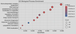
# 1. GO Enrichment (Biological Process)
ego <- enrichGO(gene = ids_biomart$entrezgene_id,
OrgDb = org.Hs.eg.db,
ont = "BP",
pAdjustMethod = "BH",
pvalueCutoff = 0.05)
dotplot(ego, showCategory=20, title="GO Biological Process Enrichment")
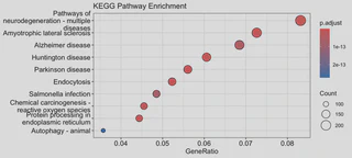
2. KEGG Pathway Enrichment
kk <- enrichKEGG(gene = ids_biomart$entrezgene_id,
                 organism = 'hsa', # 'hsa' for Homo sapiens
                 pvalueCutoff = 0.05)
dotplot(kk, showCategory=20, title="KEGG Pathway Enrichment")